With those lines from Richard II, Shakespeare unwittingly described a phenomenon in digital audio called "word clock jitter" and its detrimental effect on digitally reproduced music. "Clock jitter" refers to timing errors in analog/digital and digital/analog converters—errors that significantly degrade the musical quality of digital audio.
Clock jitter is a serious and underestimated source of sonic degradation in digital audio. Only recently has jitter begun to get the attention it deserves, both by high-end designers and audio academics. One reason jitter has been overlooked is the exceedingly difficult task of measuring such tiny time variations—on the order of tens of trillionths of a second. Consequently, there has previously been little hard information on how much jitter is actually present in high-end D/A converters. This is true despite the "jitter wars" between manufacturers who claim extraordinarily low jitter levels in their products. Another reason jitter has been ignored is the mistaken belief by some that if the ones and zeros that represent the music are correct, then digital audio must work perfectly. Getting the ones and zeros correct is only part of the equation.
Stereophile has obtained a unique instrument that allows us to measure jitter in CD players and digital processors. Not only can we quantify how much jitter is afflicting a particular D/A converter, we can look at something far more musically relevant: the jitter's frequency. Moreover, an analysis of jitter and what causes it goes a long way toward explaining the audible differences between CD transports, digital processors, and, particularly, the type of interface between transport and processor.
This article presents a basic primer on word clock jitter, explains how it affects the musical performance of digital processors, and reports the results of an investigation into the jitter performances of 11 high-end digital processors and one CD player. In addition, we are able—for the first time—to measure significant differences in jitter levels and spectra between different types of CD transport/digital processor interfaces.
We have found a general correlation between a digital processor's jitter performance and certain aspects of its musical presentation. The jitter measurements presented in this article were made on processors with whose sound I was familiar; in preparation for their reviews, each had been auditioned at matched levels for at least three weeks in my reference playback system. Because the reviews of these processors have already been published, it's possible to compare the musical impressions reported to the processors' jitter performance. Although these jitter measurements are far from the last word in quantifying a digital processor's musical performance, there is nevertheless a trend that suggests a correlation between listening and measurement.
This article will also attempt to dispel the popular notion that "bits is bits." This belief holds that if the ones and zeros in a digital audio system are the same, the sound will be the same. Proponents of this position like to draw the analogy of putting money in the bank: "your money," though merely a digital representation on magnetic tape, remains inviolate (you hope). There's a problem with this argument, however: unlike the bank's digital record on magnetic tape, digital audio data is useful only after it is converted to analog. And here is where the variability occurs. Presenting the correct ones and zeros to the DAC is only half the battle; those ones and zeros must be converted to analog with incredibly precise timing to avoid sonic degradation.
As we shall see, converting digitally represented music into analog—a process somewhat akin to turning ground beef back into steak—is far more complex and exacting than had been realized.
Sampling
To understand how even small amounts of clock jitter can have a large effect on the analog output signal, a brief tutorial on digital audio sampling is helpful.
Sampling is the process of converting a continuous event into a series of discrete events. In an analog-to-digital (A/D) converter, the continuously varying voltage that represents the analog waveform is "looked at" (sampled) at precise time intervals. In the case of the Compact Disc's 44.1kHz sampling rate, the A/D converter samples the analog waveform 44,100 times per second. For each sample, a number is assigned that represents the amplitude of the analog waveform at the sample time. This number, expressed in binary form (one or zero) and typically 16 bits long, is called a "word." The process of converting the analog signal's voltage into a value represented by a binary word is called "quantization," the effectively infinite range of values allowable in an analog system being reduced to a limited number of discrete amplitudes. Any analog value falling between two binary values is represented by the nearest one.
Sampling and quantization are the foundation of digital audio; sampling preserves the time information (as long as the sampling frequency is more than twice the highest frequency present in the analog signal) and quantization preserves the amplitude information (with a fundamental error equal to half the amplitude difference between two adjacent binary values). We won't worry about quantization here—it's the sampling process we need to understand.
The series of discrete samples generated by the A/D converter can be converted back into a continuously varying signal with a D/A converter (DAC). A DAC takes a digital word and outputs a voltage equivalent to that word, exactly the opposite function of the A/D converter (ADC). All that is required for perfect conversion (in the time domain) is that the samples be input to the DAC in the same order they were taken, and with the same timing reference. In theory, this sounds easy—just provide a stable 44.1kHz clock to the A/D converter and a stable 44.1kHz clock to the D/A converter. Voilà!—perfect digital audio.
Clock jitter
Unfortunately, it isn't that easy in practice. If the samples don't generate an analog waveform with the identical timing with which they were taken, distortion will result. These timing errors between samples are caused by variations in the clock signal that controls when the DAC converts each digital word to an analog voltage.
Let's take a closer look at how the DAC decides when to convert the digital samples to analog. In fig.1, the binary number at the left is the quantization word that represents the analog waveform's amplitude when first sampled. The bigger the number, the higher the amplitude. (This is only conceptually true—in practice the data are in twos-complement form, which uses the most significant bit or MSB at the start of the word as a sign bit, a "1" meaning that the amplitude is negative.)

Fig.1 The word-clock signal triggers the DAC to output an analog voltage equivalent to the input digital word.
The squarewave at the top of fig.1 is the "word clock," the timing signal that tells the DAC when to convert the quantization word to an analog voltage. Assuming the original sampling frequency was 44.1kHz, the word clock's frequency will also be 44.1kHz (or some multiple of 44.1kHz if the processor uses an oversampling digital filter). On the word clock's leading edge, the next sample (quantization word) is loaded into the DAC. On the word clock's falling edge, the DAC converts that quantization word to an analog voltage. This process happens 44,100 times per second (without oversampling). If the digital processor has an 8x-oversampling digital filter, the word-clock frequency will be eight times 44,100, or 352.8kHz.
It is here at the word clock that timing variations affect the analog output signal. Specifically, clock jitter is any time variation between the clock's trailing edges. Fig.2 shows a perfect clock and a jittered clock (exaggerated for clarity) (footnote 1).

Fig.2 Word-clock jitter consists either of a random variation in the pulse timing or a variation which itself has a periodic component.
Now, look what happens if the samples are reconstructed by a DAC whose word clock is jittered (fig.3). The sample amplitudes—the ones and zeros—are correct, but they're in the wrong place! The right amplitude at the wrong time is the wrong amplitude. A time variation in the word clock produces an amplitude variation in the output, causing the waveform to change shape. A change in shape of a waveform is the very definition of distortion. Remember, the word clock tells the DAC when to convert the audio sample to an analog voltage; any variations in its accuracy will produce an analog-like variability in the final output signal—the music.
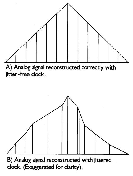
Fig.3 Analog waveform is constructed correctly with a jitter-free word clock (top); word-clock jitter results in a distortion of the analog waveform's shape (exaggerated for clarity).
There's more. Clock jitter can raise the noise floor of a digital converter, reducing resolution, and can introduce spurious artifacts. If the jitter has a random distribution (called "white jitter" because of its similarity to white noise), the noise floor will rise. If, however, the word clock is jittered at a specific frequency (ie, periodic jitter), artifacts will appear in the analog output as sidebands on either side of the audio signal frequency being converted to analog. It is these periodic artifacts that are the most sonically detrimental; they bear no harmonic relationship to the music and may be responsible for the hardness and glare often heard from digital audio.
These principles were described in JA's computer simulations of the effects of different types and amounts of jitter in Vol.13 No.12; I've included three of his plots here. Fig.4 is a spectral analysis of a simulated DAC output when reproducing a full-scale, 10kHz sinewave with a jitter-free clock. Fig.5 is the same measurement, but with two nanoseconds (2ns or 2 billionths of a second) of white jitter added—note the higher noise floor. Fig.6 shows the effect of 2ns of jitter with a frequency of 1kHz. The last plot reveals the presence of discrete frequency sidebands on either side of the test signal caused by jitter of a specific frequency. The amplitude of these artifacts is a function of the input signal level and frequency; the higher the signal level and frequency, the higher the sideband amplitude in the analog output signal (footnote 2).

Fig.4 Audio-band spectrum of jitter-free 16-bit digital data representing a 10kHz sinewave at 0dBFS (linear frequency scale).

Fig.5 Audio-band spectrum of 16-bit digital data representing a 10kHz sinewave at 0dBFS afflicted with 2ns p-p of white-noise jitter (linear frequency scale). Note rise of approximately 12dB in the noise floor compared with fig.4, which represents a significant 2dB loss of signal resolution.
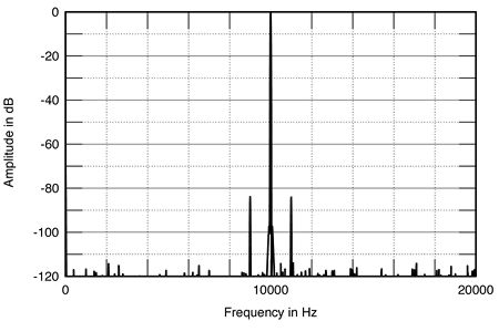
Fig.6 Audio-band spectrum of 16-bit digital data representing a 10kHz sinewave at 0dBFS afflicted with 2ns p-p of sinusoidal jitter at 1kHz (linear frequency scale). Note addition of sidebands at 9kHz and 11kHz compared with fig.4, though the noise floor remains at the 16-bit level.
How much jitter is audible? In theory, a 16-bit converter must have less than 100 picoseconds (ps) of clock jitter if the signal/noise ratio isn't to be compromised. (There are 1000ps in a nanosecond; 1000ns in a microsecond; 1000µs in a millisecond; and 1000ms in a second.) Twenty-bit conversion requires much greater accuracy, on the order of 8ps. 100ps is one-tenth of a billionth of a second (1/1010s), about the same amount of time it takes light to travel an inch. Moreover, this maximum allowable figure of 100ps assumes the jitter is random (white) in character, without a specific frequency which would be sonically less benign. Clearly, extraordinary precision is required for accurate conversion (see Sidebar).
Where does clock jitter originate? The primary source is the interface between a CD transport and a digital processor. The S/PDIF (Sony/Philips Digital Interface Format) signal that connects the two has the master clock signal embedded in it (it is more accurate to say the audio data are embedded in the clock). The digital processor recovers this clock signal at the input receiver chip (usually the Yamaha YM3623B, Philips SAA7274, or the new Crystal CS8412).
The typical method of separating the clock from the data and creating a new clock with a phase-locked loop (PLL) produces lots of jitter. In a standard implementation, the Yamaha chip produces a clock with 3-5 nanoseconds of jitter, about 30 to 50 times the 100ps requirement for accurate 16-bit conversion (the new Crystal CS8412 input receiver in its "C" incarnation reportedly has 150ps of clock jitter). Even if the clock is recovered with low jitter, just about everything inside a digital processor introduces clock jitter: noise from digital circuitry, processing by integrated circuits—even the inductance and capacitance of a printed circuit board trace will lead to jitter.
It's important to note that the only point where jitter matters is at the DAC's word-clock input. A clock that is recovered perfectly and degraded before it gets to the DAC is no better than a high-jitter recovery circuit that is protected from additional jitter on its way to the DAC. Conversely, a highly jittered clock can be cleaned up just before the DAC with no penalty (footnote 3).
Logic induced modulation (LIM)
There are two other significant sources of jitter in D/A converters. The first mechanism was recently discovered by Ed Meitner of Museatex and Robert Gendron, formerly a DAC designer at Analog Devices and now at Museatex. This jitter-inducing phenomenon, called Logic Induced Modulation (LIM), was discovered only after Meitner and Gendron invented a measurement system that revealed its existence. This measurement tool, called the LIM Detector, reveals not only how much clock jitter is present in a digital processor, but also displays its spectral distribution when connected to a spectrum analyzer or FFT machine. The jitter's spectral content—and whether or not it is random or composed of discrete frequencies—is much more important sonically than the overall amount of jitter. Two digital processors could each claim, say, 350ps of jitter, but the processor whose word clock was jittered at a specific frequency would likely suffer from a greater amount of sonic degradation than the other processor which had the same RMS level of random jitter. More on this later.
It's worth looking at Logic Induced Modulation in detail; the phenomenon is fascinating:
LIM is a mechanism by which the digital code representing an audio signal modulates (jitters) the clock signal. If a digital processor is driven by the code representing a 1kHz sinewave, the clock will be jittered at a frequency of 1kHz. Put in 10kHz, and jitter with a frequency of 10kHz will appear on the clock. Remember, jitter with a specific frequency is much more sonically pernicious than random-frequency jitter.
Here's how LIM is generated. In an integrated circuit (IC), there are many thousands of transistors running off the same +5V (usually) power-supply rail. When an IC is processing the code representing a 1kHz sinewave, for example, those thousands of transistors are turning on and off in a pattern repeating 1000 times per second. The current demands of all those transistors turning on together modulates the power-supply rail at the frequency of the audio signal. Just as the lights in a house dim momentarily when the refrigerator motor turns on, the +5V power-supply rail droops under sudden current demand from the chip's transistors. The analog audio signal thus appears on the IC's power-supply rail.
Now, the transition between a logic "0" and a logic "1" occurs at the leading edge of a squarewave. The precise point along the leading edge at which the circuit decides that a "1" is present is determined by the power-supply voltage reference. If that voltage fluctuates, the precise time along the leading edge at which the circuit recognizes a "1" will also fluctuate—in perfect synchronization with the power-supply voltage modulation. This uncertainty in the timing of the logic transitions induces jitter on the clock—at the same frequency as the audio signal the IC is processing. Put in the code representing 1kHz and the IC's power supply will be modulated at 1kHz, which in turn causes jitter on the clock at 1kHz. According to Meitner, it is possible to AC-couple a high-gain amplifier to the digital power-supply rail and hear the music the processor is decoding.
This astonishing phenomenon was discovered quite by accident after Meitner and Gendron designed the device to display the jitter's spectral distribution. When they put in a 1kHz digital signal, the jitter had a frequency of 1kHz with its associated harmonics. (footnote 4, footnote 5)
There is another mechanism by which clock jitter correlated with the audio signal is created. This phenomenon, described by Chris Dunn and Dr. Malcolm Hawksford in their paper presented at the Fall 1992 Audio Engineering Society convention (and alluded to in the Meitner/Gendron paper), occurs in the AES/EBU or S/PDIF interface between a transport and a digital processor. Specifically, they showed that when the interface is band-limited, clock jitter with the same frequency as the audio signal being transmitted is produced in the recovered clock at the digital processor. Although this phenomenon produces the same type of signal-correlated jitter as LIM, it is a completely different mechanism. A more complete discussion of Dunn's and Hawksford's significant paper [reprinted in Stereophile in March 1996 (Vol.19 No.3) as "Bits is Bits?"—Ed.] can be found in my AES convention report in next month's "Industry Update." (footnote 6)
Measuring clock jitter
Museatex has made the LIM Detector available to anyone who wants to buy one. Stereophile jumped at the chance (see Sidebar).
First, you have to open the processor's chassis and find the DAC's word-clock pin with a conventional oscilloscope and probe. The probe hooked up to the word-clock signal is then connected to the input of the LIMD and the LIMD is tuned to that word clock using preset frequency settings. To look at the spectrum of any processor's word clock (up to 20kHz), we fed the LIMD's analog output to our Audio Precision System One Dual Domain to create FFT-derived spectral analysis plots. A one-third-octave analyzer can also be used, though this gives less frequency resolution, of course. If the output of the LIMD is connected to an RMS-reading voltmeter, the overall jitter level can be read as an AC voltage. Knowing how many millivolts are equivalent to how many picoseconds of jitter—the LIMD output voltage also depends on the sampling frequency—allows the jitter to be easily calculated.
The measurements of digital-processor clock jitter included in this article thus include the processor's overall jitter level expressed in picoseconds and a plot of the jitter's spectral distribution. The latter is scaled according to the RMS level—0dB is equivalent to 226.7ns of jitter—so that spectra for different processors can be readily compared.
Before getting to the measurement results, a quick description of how the LIMD works is useful. Like all brilliant inventions, the technique is simple and obvious—after you've been told how it works.
A jittered clock can be considered as a constant carrier signal which has been frequency-modulated (FM). The jitter components can therefore be separated from the clock by an FM demodulator—just like those found in all FM tuners. In the LIMD, once it has been correctly tuned to the word-clock frequency, an FM demodulator removes the clock signal, leaving only the audio-band jitter components—which can be measured as a voltage or output for spectral analysis.
I have no doubt that many manufacturers of the digital processors tested for this article will question the test methodology and results. Some claim extraordinarily low jitter in their products—claims that were not confirmed by my measurements. This disparity can arise because there is no standard method of measuring jitter. When I'm told by a manufacturer that his product has "less than 70ps of jitter," my first question is, "How do you measure 70ps?" The response is often less than adequate: "We calculate it mathematically" is a common reply. Moreover, some jitter measurements attempt to measure jitter indirectly—as a function of the rise in the noise floor, for example—rather than looking directly at the word clock.
At any rate, if the absolute levels presented in this article are in error, the relative differences between processors will still be correct. If anyone can demonstrate a better method of measuring jitter, I'm all ears.